The Normal Distribution

Introduction

This is the fourth post in my statistics series and this time we are going to focus on the normal distribution.
It is arguably the most important probability distribution in statistics and the key to understanding and modelling many phenomena. In this post, we will see what the normal is, how it can be manipulated and how to calculate areas under it.

(Brief) History lesson

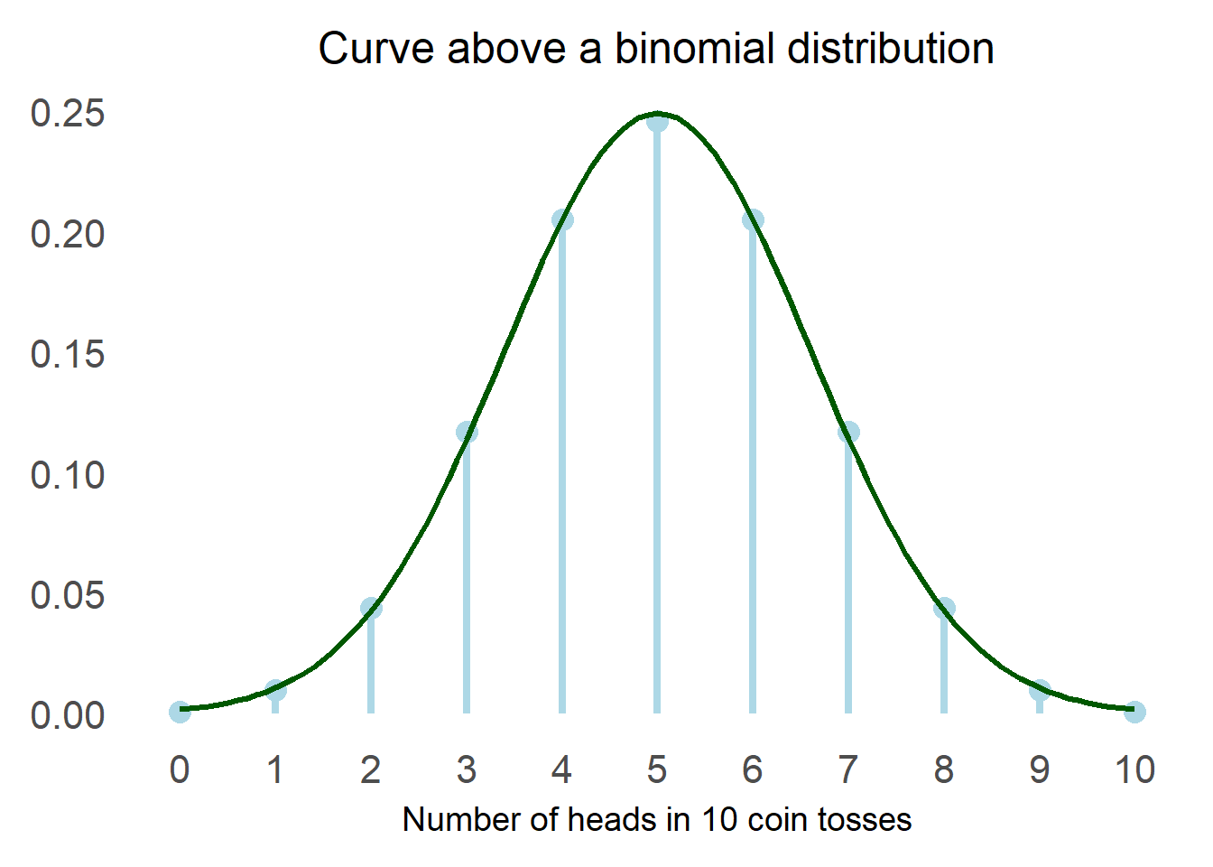
The first person to “discover” the normal distribution was Abraham de Moivre, an 18th century statistician. He was trying to find a good way to estimate probabilities in gambling and he came across the normal distribution as the limiting curve for the binomial.
In simpler terms, he noticed that if he plotted the number of heads that came out in repeated coin tosses he could draw a particular curve above the distribution. What he probably noticed looked like this:

After that first occurrence, it was observed in various calculations but it was formalised by Adrain and Gauss at the beginning of the 19th century, and this is how we came to this lovely formula:

$$ \large f_X(x) = \frac 1 {\sigma \sqrt{2\pi}}e^{-\frac 1 2 (\frac {x-\mu} {\sigma})^2} $$

This is the probability density function for a generic normal distribution $$ Ν(\mu, \sigma^2) $$ while the probability density function for the standard normal distribution (mean = 0 and variance = 1) is:

$$ \large \phi(x) = \frac 1 {\sqrt{2\pi}}e^{-\frac {x^2} 2 } $$

Thankfully we have computers to do the calculations for us and we do not need to work too much with these formulas.

Calculating probabilities of a standard normal

For many applications (including statistics) we need to be able to calculate probabilities under the standard normal in order to answer questions such as:
“What is the probability that a value of a standard normal will be less than -1?"
The first step is to translate this question into a mathematical formulation. What we are looking for is: $$ P[Z \le -1] $$

Lets visualise the probability:

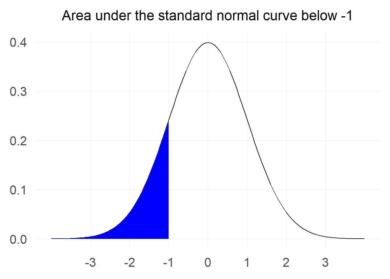
The area marked in blue corresponds to the probability that we are interested in. To calculate such area we can use the lessons from calculus and integrate the probability density function from negative infinity until -1.
All good so far, but now we hit a big obstacle: There is no closed form solution for the integral of the normal distribution. Fortunately, we have various numerical approximations for it that can help us perform the calculation.

To obtain a result, we can use the pnorm function in R (or equivalent functions in other statistical software) or we could also use a standard table which brings us to the following result:

The probability that a value from a standard normal distribution will be less than -1 is: 0.159

Cumulative Distribution Function

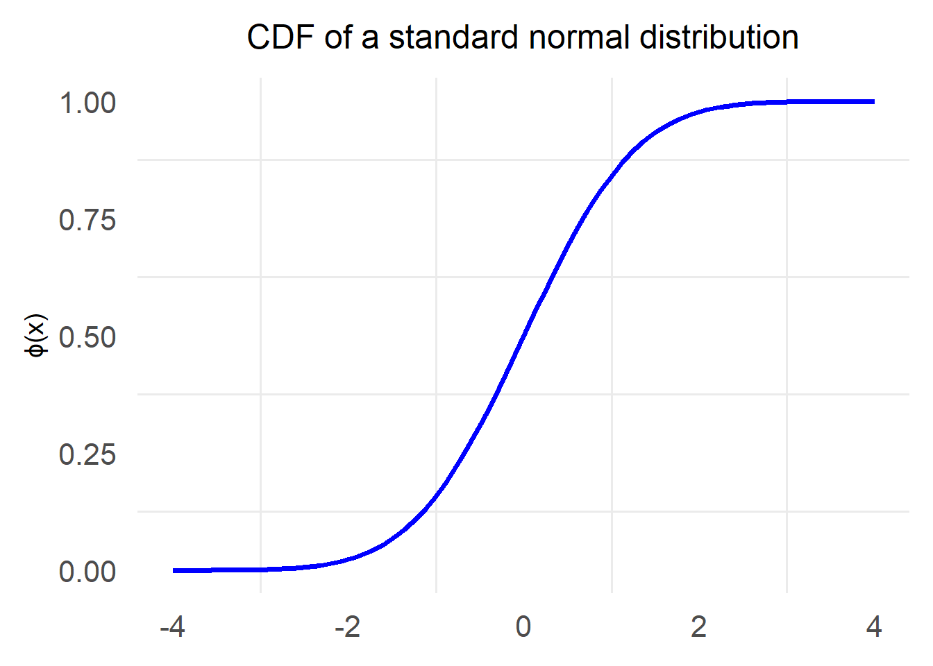
This operation of calculating the probability that a sample from a distribution will fall below certain value x is very common and there is a specific function that takes as input such a value x and returns the probability $$ P[X \le x] $$ This function is called Cumulative Distribution Function or CDF for short and is defined as follows: $$ F_X(x) = P[X \le x] $$

The typical notation for the CDF of the standard normal distribution is to use the letter Φ: $$ \Phi(x) = P[Z \le x] $$

Properties of the CDF

Before moving on, it’s good to try and understand some of the properties of the CDF:

$$ 0 \le \Phi(x) \le 1 $$

This one is quite understandable given that the CDF returns a probability and as we know any probability is bounded between 0 and 1.

$$ \lim\limits_{x \rarr -\infty}\Phi(x)=0$$ This property simply states that the probability that a sample value from a standard normal will be less than a very small number is essentially zero. To be even more practical about it, we can use pnorm to calculate the probability that the value of a standard normal will fall below -5:

The probability that a value from a standard normal distribution will be less than -5 is: 0.0000002866516

Clearly we do not need to reach negative infinity for the probability to be essentially zero.

$$ \lim\limits_{x \rarr \infty}\Phi(x)=1$$

The other side of the property above, the probability that a value from a standard normal will be below certain gigantic number is essentially 1. Again let’s be practical and use pnorm to calculate what is the probability that the value of a standard normal will fall below 5:

The probability that a value from a standard normal distribution will be less than 5 is: 0.9999997

Similarly to the previous property, it becomes obvious that we do not need to reach infinity for the probability to be essentially equal to 1.

Using this newly acquired notation we can rewrite our original computation $$ P[Z \le -1] = \Phi(-1) $$

All probability calculations for a standard normal that we might need can be performed by employing some clever tricks using its CDF and symmetry.

Probability of a value above x

We might want to calculate what is the probability that we will get a value greater than 2: $$ P[X \ge 2] $$ Let’s first visualise the probability we are interested in:

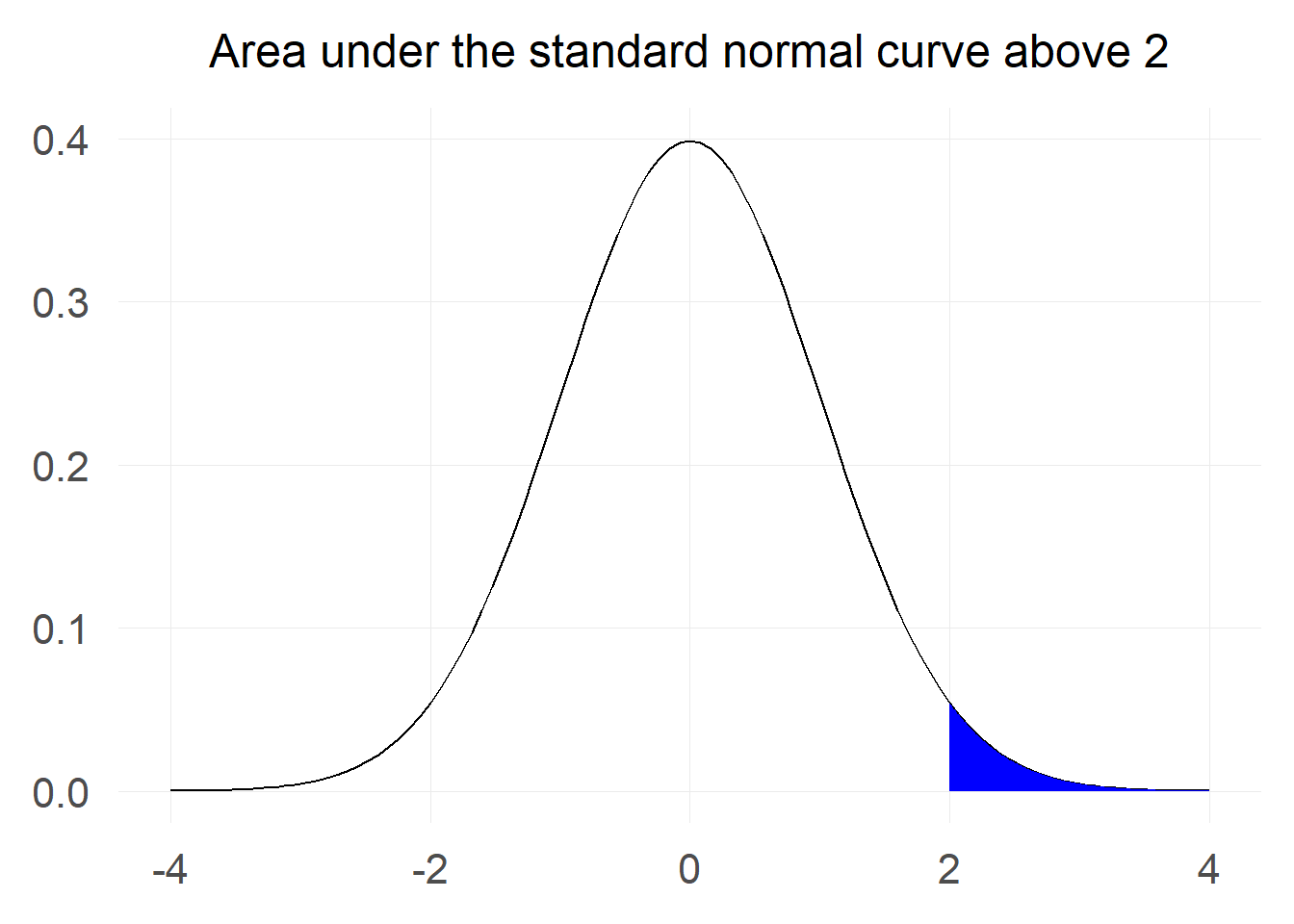
At first this looks challenging as we only have information for probabilities of the sort $$ P[Z \le x] $$ but not for $$ P[Z \ge x] $$

Using symmetry

The first trick we can use is the fact that the standard normal distribution is symmetric around 0, which means that the probability of a value being greater than 2 is the same as the probability of a value being less than -2.

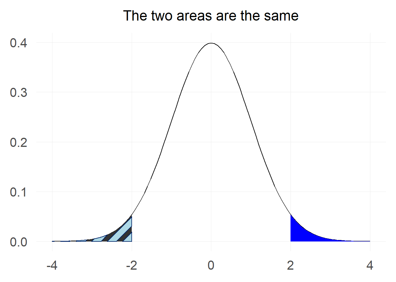
In mathematical notation this can be written as $$ P[Z \ge 2] = P[Z \le -2] = \Phi(-2) $$

Using total probability

We know from the basics of probability that the total probability under the standard normal curve is equal to 1. We can make use of this fact in order to transform the calculation.

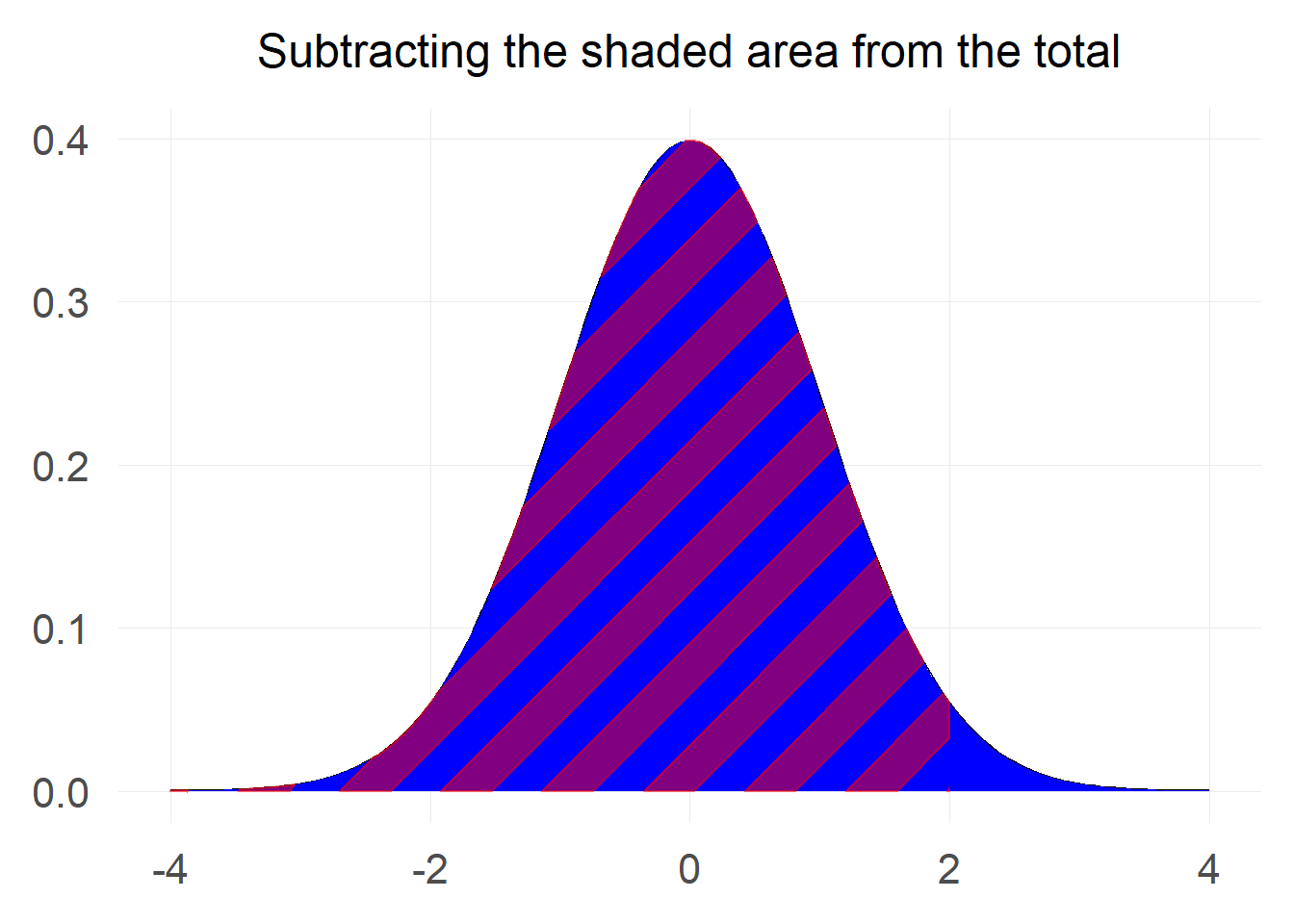
$$ P[Z \ge 2] = 1-P[Z \le 2] = 1 - \Phi(2) $$

Probability of a value between x1 and x2

Now comes the trickier calculation:
“What is the probability that a value from a standard normal will be between -2 and 1?"
Let’s start by visualising the area we are interested in.

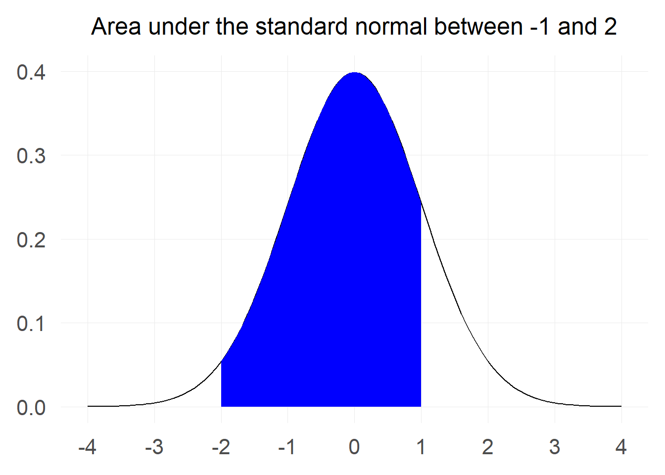
We can do some minor adjustments to the last trick we used with the total probability in order to make the calculation. If you look at the chart carefully you will notice that the probability we are interested in is the probablity that a value is below 1 minus the probability that a value is below -2. Pictorially:

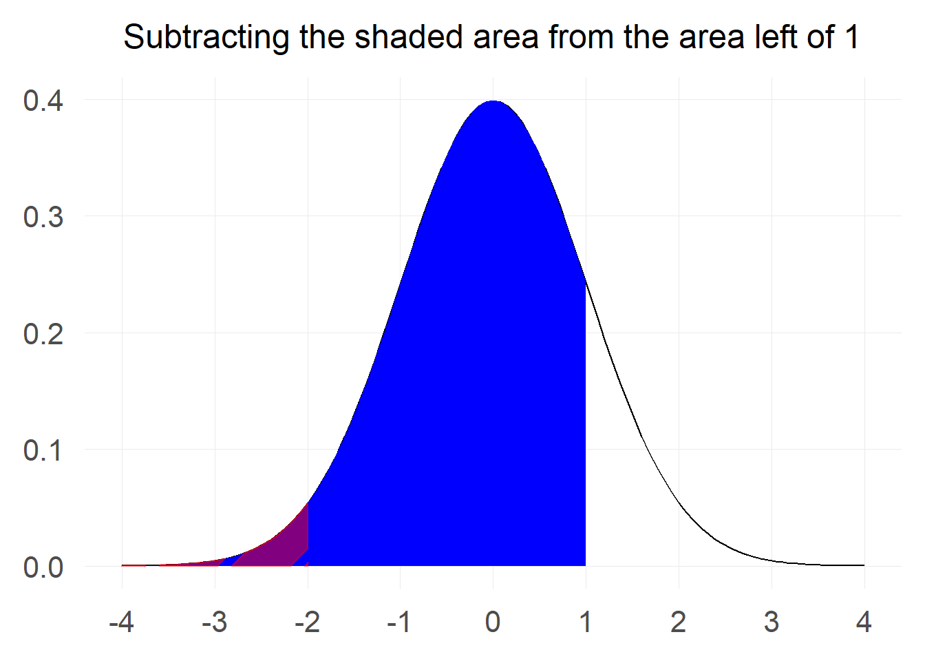
$$ P[-2 \le Z \le 1] = P[Z \le 1] - P[Z \le -2] = \Phi(1) - \Phi(-2) $$

Reversing the procedure - How to find X

So far we have looked into cases where we had to find a probability based on certain values of x.
What should we do if someone reverses the problem and tells us to find x such that the probability of a value from standard normal falling below x is equal to a certain number. More succinctly:

$$ \text{Find x such that:}\ P[Z \le x]=\Phi(x) = 0.159 $$

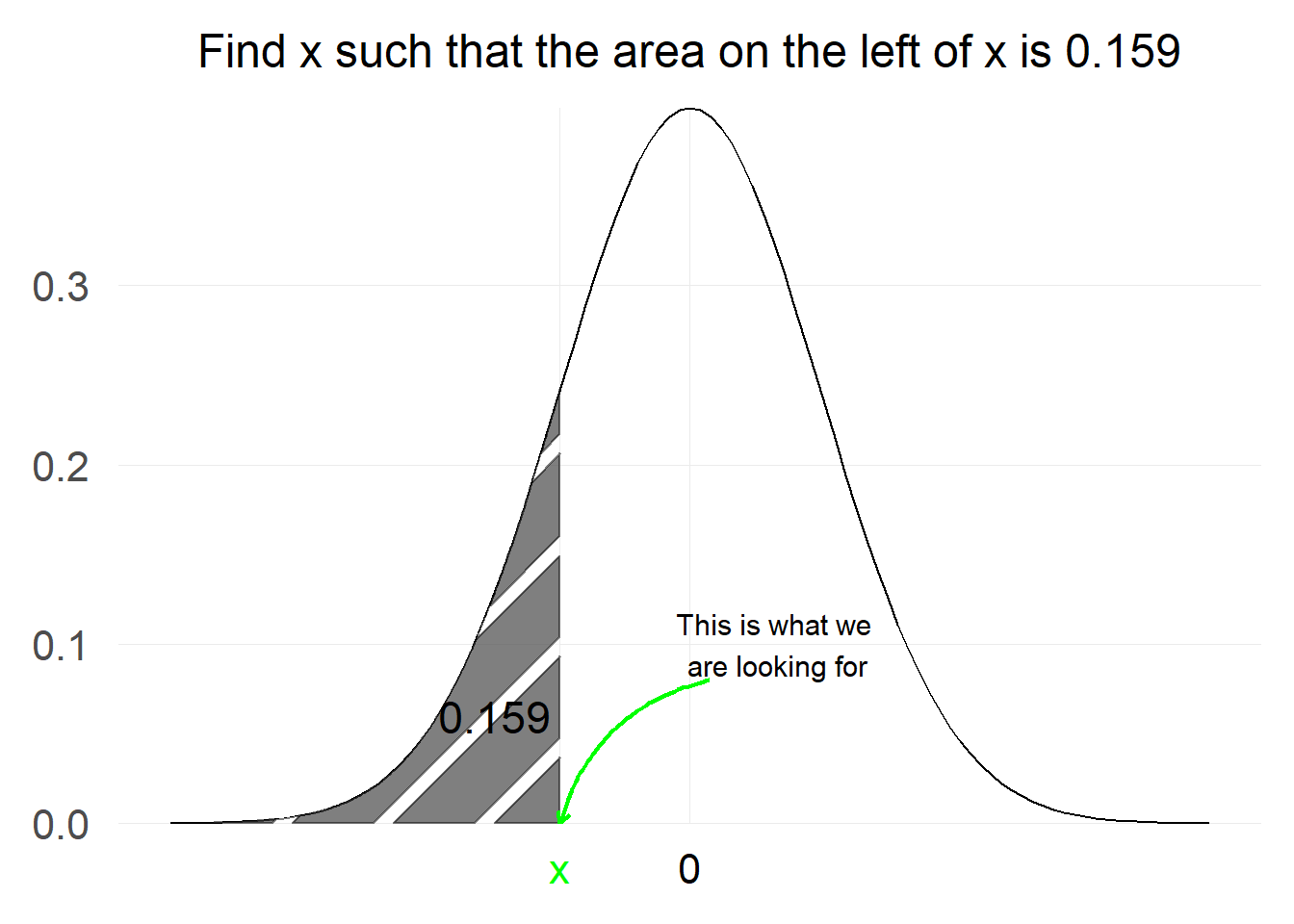
Essentially, what we are trying to achieve here is the inverse of what we were trying to do before.
Previously we used the CDF in order to calculate the probability on the left hand side of x.
Now we know the probability and we are trying to find x such that the probability on the left of it is equal to the known value.

Luckily there is a function we can use that does exactly this and it is called the Inverse Distribution Function. Provided that both the CDF and the inverse exist the following equation holds:

$$ F_X(x) = q \Harr F^{-1}(q) = x$$

To find the value of x we are looking for we can use the qnorm function in R (or equivalent functions in other statistical software) or we could also use a standard table:

The value x such that the probability on the left side of x is 0.159 is: -1

Why would these calculations be useful?

It is important to mention why these calculations are relevant for practical purposes. After all, the normal distribution is simply one distribution, there are countless others.
The main reason these calculations are needed is the Central Limit Theorem, which allows us to describe the normalised distribution of the sample mean for any arbitrary distribution by using the normal distribution.
In practical terms, in order to perform hypothesis testing, calculate confidence intervals and many other computations we need to be able to calculate probabilities for the distribution we are interested in. Most of the time, this distribution is either (i) unknown or (ii) difficult to manipulate. Therefore, we resort to the CLT in order to be able to work with the standard normal distribution and draw conclusions for the original distribution as we shall see in future posts.

Useful resources

https://en.wikipedia.org/wiki/Normal_distribution https://onlinestatbook.com/2/normal_distribution/history_normal.html https://en.wikipedia.org/wiki/Cumulative_distribution_function https://en.wikipedia.org/wiki/Cumulative_distribution_function#Inverse_distribution_function_(quantile_function)