Estimators
in statistics
December 12, 2021
Introduction
This is the third post in my statistics series and today we are going to talk about estimators. What they are, why would we use them and what are some desirable properties that we would like them to have.
Definition
An estimator is a rule for calculating an estimate of a given quantity based on observed data
Essentially what we learn from the definition is that an estimator is a recipe that takes in observed data and returns an estimate which we hope is a good approximation of a given quantity.
Pictorially, the process looks like this:
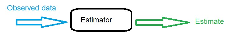
Notation notice
Estimator: The recipe to go from the observed data to the estimate
Estimate: The value that gets produced from the estimator given observed data
Estimand: The quantity that we are trying to estimate using the estimator
But before we start going into more detail, why would we need an estimator in the first place? We will examine the usefulness of estimators and understand their properties through an example.
How many people pass by in front of my house?
Let’s say that I spend my time observing the people that pass by in front of my house. Sometimes many people pass by and sometimes few, but this is not specific enough for me. Given that I am into statistics, I decide that I would like a better way to describe the number of passers-by.
It is good to start with some specifications about the process:
- I only observe passers-by during work days between 9-12 and 2-5. This means that there are no fluctuations due to holidays or shopping hours that can change the numbers significantly.
- I am counting people per hour. (I could have chosen a different time interval, the hour is arbitrary)
Time to model
I have kept track of 10 hours of people passing by so let’s have a look at the data.
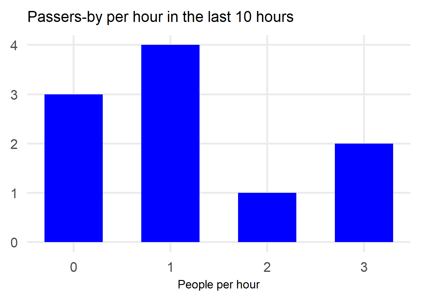
Based on the data we observe the following:
- 0 people passed outside my house in 3 out of the 10 hours that I kept track
- 1 person passed by in 4 out of the 10 hours
- 2 people passed by in 1 out of the 10 hours
- 3 people passed by in 2 out of the 10 hours
My first try at modelling would be to use relative frequency. Based on this small sample, we could say that the probability that 0 people will pass by the house in the next hour is 3/10=0.3, the probability that 1 person will pass by the house is 4/10=0.4 and so on.
There are merits to this method but also downsides:
| + | - |
|---|---|
| No assumptions about distributions | Many parameters need to be estimated (P(0), P(1), P(2), etc.) which requires lots of data |
| Easy to calculate given data | Tough to assign probability to unlikely events |
The last negative might be a bit confusing so let me give an example:
What happens if the actual chance that 5 people pass by my house is 1/1000? We would have to wait (on average) a lot of days to see this event occurring. Otherwise we would simply give it a probability of 0.
The other option we have is to assume that the number of passers-by is following a certain statistical distribution. Again, there are pros and cons to this approach:
| + | - |
|---|---|
| Few parameters to calculate depending on the distribution | Depending on the problem, it can be tough to pick the statistical distribution |
| Easy to make predictions for unseen events | The data could in reality differ a lot from the chosen distribution |
Given that this is a post about estimators, we will have to pick a distribution for sure 😂
Which family of statistical distributions should we pick?
Based on problem construction we can eliminate some distributions:
- The distribution has to be discrete as we are counting people
- It has to take values in the non-negative integers
That’s a good start, but really it does not help us thaaat much.
To get more help we could do:
- Check in previous studies about statistical distributions selected for similar problems
- Look at the 10 data points we have to perhaps eliminate some distributions
The most common statistical distribution that is selected for modelling arrival rates (which is the type of problem we have here) is the Poisson. Just as a reminder the distribution looks like this:
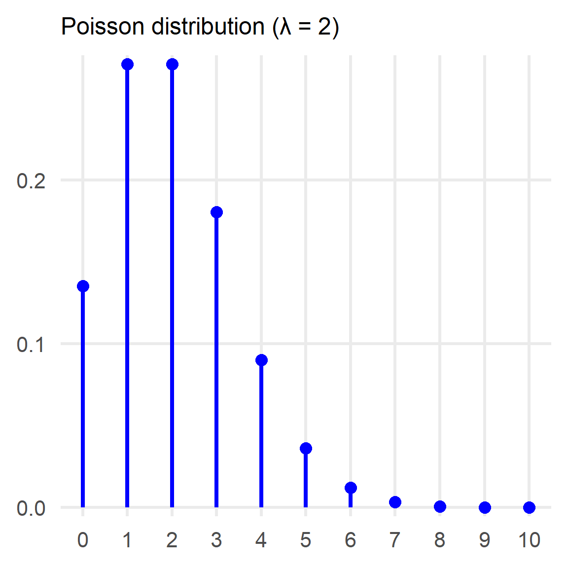
Furthermore, we know that: $$ E[Pois(\lambda)] = \lambda\ \text{and}\ Var(Pois(\lambda))=\lambda $$
A version of the Poisson distribution does look plausible given the problem and the small sample of data that we have.
⚠️ In reality it is highly unlikely that we will find a distribution that matches our data perfectly. What we are trying to achieve is to find a distribution that gives a good approximation.
So we can conclude the following regarding our modelling:
- We are assuming that the observed values in the sample are all coming from a Poisson(λ) distribution
- We are assuming that the observed values are independent (reasonable assumption for passers-by)
Mathematically: $$ X_1, X_2, …, X_n \sim Pois(\lambda)\ i.i.d. $$ where the Xi correspond to the number of passers-by in the first, second, third…etc. hour.
Which is the correct parameter?
We decided on a Poisson distribution, but now comes the second question: Which one?
There are infinite Poisson distributions depending on the parameter λ that we choose.
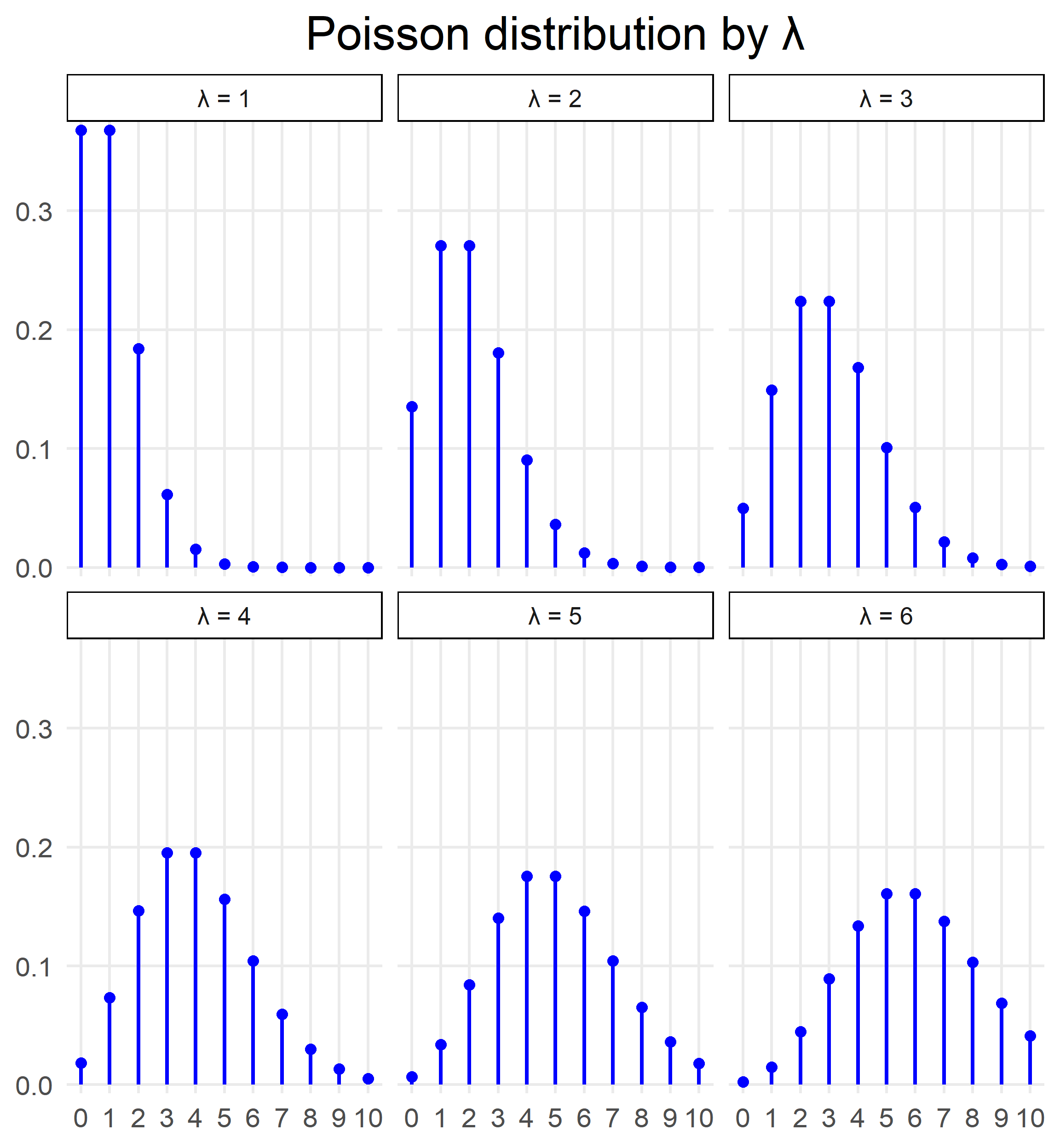
This is the part where estimators come in. We need an estimator to estimate the parameter λ of the Poisson distribution that we picked.
Let’s select some estimators
I will showcase some desirable estimator properties for 3 possible estimators (the estimator is marked with a hat on top of it):
$$ \text{Estimator 1: } \widehat{\lambda_1} = \overline{X_n} $$ $$ \text{Estimator 2: } \widehat{\lambda_2} = X_1 $$ $$ \text{Estimator 3: } \widehat{\lambda_3} = 4 $$
All three estimators are valid (a valid estimator is a statistic (any function of the data) that does not depend on the parameter we are trying to estimate, in this case λ), but the estimate that gets produced by each one of them is different:
The first estimator takes the observed values and outputs the sample mean.
The second estimator produces as an estimate the first value in the observed sample.
The third estimator produces as an estimate the value 4 regardless of what we have observed.
Bias of an estimator
The bias of an estimator is the difference between this estimator’s expected value and the true value of the parameter being estimated
Ideally, we would like our estimator to be unbiased, which means that we hope that on average (expected value) it is equal to the parameter we are trying to estimate (λ in this case, the estimand).
Calculating expectation
Expectation of estimator #1:
$$ E[\widehat{\lambda_1}] = E[\overline{X_n}] = E[X] = \lambda$$ Expectation of estimator #2:
$$ E[\widehat{\lambda_2}] = E[X_1] = E[X] = \lambda$$ Expectation of estimator #3:
$$ E[\widehat{\lambda_3}] = E[4] = 4$$
Calculating bias
Bias of estimator #1:
$$ Bias(\widehat{\lambda_1}) = E[\widehat{\lambda_1}] - \lambda = \lambda-\lambda=0$$ Bias of estimator #2:
$$ Bias(\widehat{\lambda_2}) = E[\widehat{\lambda_2}] - \lambda = \lambda-\lambda=0$$ Bias of estimator #3:
$$ Bias(\widehat{\lambda_3}) = E[\widehat{\lambda_3}] - \lambda = 4 - \lambda$$
Variance of an estimator
The variance of an estimator is a very important property. Low variance estimators are to be preferred (as long as their distribution is reasonably close to the estimand!). Calculating the variance is very straightforward, we are simply using the same formulas as for any other random variable.
Variance of estimator #1: $$ Var[\widehat{\lambda_1}] = Var[\overline{X_n}] = \frac {Var(X)} n = \frac {\lambda} n$$ Variance of estimator #2: $$ Var[\widehat{\lambda_2}] = Var[X_1] = Var[X] = \lambda$$ Variance of estimator #3: $$ Var[\widehat{\lambda_3}] = Var[4] = 0$$
Consistency of an estimator
A consistent estimator is an estimator having the property that as the number of observations increases indefinitely, the resulting sequence of estimates converges in probability to the quantity we are trying to estimate.
Concretely for our example this means that the more hours of data we collect, the more reliable a consistent estimator will become and with sufficiently large number of hours (reaching infinity) the distribution of the consistent estimator will be very tightly concentrated around the estimand.
In mathematical terms: $$ \large \widehat{\lambda} \xrightarrow[n \rarr \infty]{\Bbb{P}} \lambda $$
Let’s see the consistency of our three estimators:
Consistency check for estimator #1: $$ \large \widehat{\lambda_1} = \overline{X_n}\xrightarrow[n \rarr \infty]{\Bbb{P}} E[X]=\lambda $$
This relationship holds because of the Law of Large Numbers which states that for sufficiently large n the average of the results obtained from a large number of trials (sample mean) should be close to the expected value. In this case, the expected value of X is also the quantity we are trying to estimate and therefore the estimator is consistent.
Consistency check for estimator #2:
The probability distribution of the second estimator is unaffected by the number of points we collect. Therefore, it is not consistent.
Consistency check for estimator #3:
The distribution of the 3rd estimator remains constant and equal to 4. This estimator is not consistent.
Putting together the results
| Estimator | Bias | Variance | Consistency |
|---|---|---|---|
| #1 | 0 | λ/n | Yes |
| #2 | 0 | λ | No |
| #3 | 4-λ | 0 | No |
Looking at the table, we can see that the first estimator (the sample mean) is the one to be preferred as it has:
- No bias
- Variance that decreases (and tends to 0) as the number of observations increases
- Consistency
Other desireable properties
The 3 properties that I described are generally accepted as the most important ones but depending on the problem another 2 factors could play an important role:
- Robustness: Robust estimators produce reliable estimates even when the modelling assumptions are not 100% accurate.
- Computational complexity: An estimator that can be easily computed might be preferable to one with slightly better properties that is very hard to compute.
Conclusion
We saw in this post what is the reasoning behind trying to find estimators. While it is very easy to pick an estimator (as we saw it can be almost any function that does not depend on the estimand), finding a good one requires some effort. In the next statistics posts we are going to see how to pick them.
- Posted on:
- December 12, 2021
- Length:
- 8 minute read, 1685 words
- Categories:
- statistics
- Tags:
- statistics