The Law of Large Numbers

Introduction

I decided after years of struggling to remember statistical concepts that I have to try to explain them so that:

1. I am forced to understand them better 😄
2. Anybody can read and comment which can offer useful insights that I might have missed
3. I will be able to come back to my explanation once I forget the concept

Please note that this is not a very math heavy collection of posts, my goal is to get a better intuitive understanding of the concepts.
With all that being said, this is the first post in my statistics series and it is about the Law of Large Numbers!

Definition

The Law of Large Numbers states that the average of the results obtained from a large number of trials should be close to the expected value and will tend to become closer to the expected value as more trials are performed

Let’s try to map the words in the definition to mathematical constructions.

Large number of trials

Here we assume that we are doing multiple trials coming from the same underlying probability distribution.

We can model these trials as n random variables: $$ X_1, X_2, …, X_n $$

These variables are identically distributed (so all follow the same distribution) and they are independent (knowledge about the outcome of one of them does not provide any information about the others). More trials means higher n (larger sample size).

Average of the results

The mathematical representation of the average of the results is the sample mean or sample average: $$ \overline{X_n} = \frac {X_1 + X_2+…+X_n} n $$

Expected value

The expected value of a random variable can be thought of intuitively as the arithmetic mean of a large number of independent realizations of X. (This is not the topic of this post so I will not go into more detail)
The expectation of our random variables is the following:

$$ E[X_1] = E[X_2] = … = E[X_n] = E[X] = \mu $$

Unfortunately, in many scenarios we do not know what value μ takes therefore we need something to estimate it.
This is where the Law of Large Numbers comes in and tells us that the sample mean should be close to the expected value and this “closeness” increases with the number of trials.
Stated in a mathematical formulation:

$$ \overline{X_n} \xrightarrow[n\rarr \infty]{P} E[X] $$

In action

We are going to see three examples of the Law of Large Numbers for the following three distributions:

1. Standard normal (Continuous random variable)
2. Binomial (Discrete random variable)
3. My own distribution (I have not coined it yet but it’s happening! 😄) (Mixed random variable)

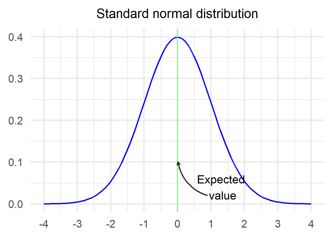
1. Samples from a standard normal distribution

In our first example, we assume the following:

$$ X_1, X_2, …, X_n \thicksim N(0,1)\ i.i.d.$$

Just as a reminder, this is what the standard normal looks like:

Let’s see how the sample mean changes as the sample size increases.

In the annimated chart above we can see how the sample average changes as sample size increases. At the beginning it is far from the expected value (marked in green) but as the number of samples grows larger it gets closer and closer.

2. Unbiased coin flip

The next example is a very typical one, it is the toss of an unbiased coin. In particular, we model the toss of an unbiased coin by using a Bernoulli distribution with the following mapping:

• Heads: The outcome of the Bernoulli is 1
• Tails: The outcome of the Bernoulli is 0

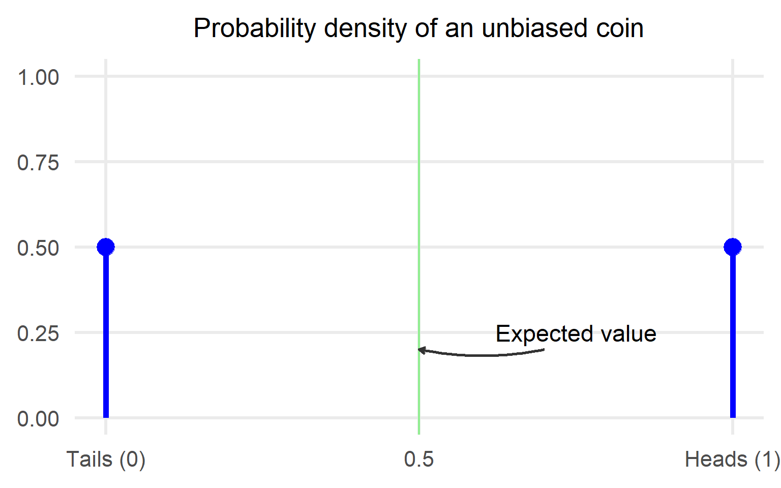
The expected value of an unbiased coin toss is 0.5 or equivalently phrased you expect to get half heads and half tails. Mathematically, we assume the following:

$$ X_1, X_2, …, X_n \thicksim Ber(0.5)\ i.i.d.$$

Let’s see how the sample mean changes as the number of samples increases.

Again we see that as the number of samples increases, the sample mean approaches the expected value.

3. Random distribution I came up with

As a last example, we are going to illustrate the Law of Large numbers for an arbitrary distribution that I came up with.
Let’s make this even more interesting and pick a mixed distribution. Just as a reminder, a mixed distribution is a distribution that is neither continuous nor discrete. In some parts, it is continuous and in some parts it is discrete.

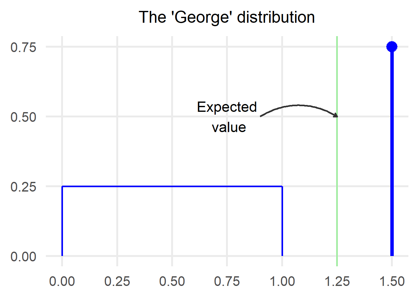
As we can see from the plot above, the ‘George’ distribution consists of the following two parts:

1. Continuous: We have a uniform from 0 to 1 with a height of 0.25
2. Discrete: There is a 0.75 probability that a sample from the ‘George’ will take a value of 1.5

It’s a good idea to check if the total probability sums to 1:

$$ Total\ probability = 0.25*1 (rectangle\ area) + 0.75 = 1$$

We take again 500 samples from this distribution. Let’s see how the sample mean changes as the sample size increases.

Ok clearly something went terribly wrong! Here I have been plotting throughout this blog showing you that the red line eventually gets really really close to the green one but clearly it is not the case!
Did I miscalculate the expectation of my own distribution or is the Law of Large Numbers a hoax?

Surprisingly neither!

The Law of Large Numbers does not state anything about the speed of convergence. It only states that as the number of trials gets larger, the sample mean will get closer and closer to the expected value.
Let’s try it again but with a higher number of samples this time:

We can clearly see that it took longer for the sample mean to reach the expected value in my distribution but it did reach it nonetheless!

Law of Large Numbers vindicated!

Why is this cool?

The Law of Large Numbers is a fundamental building block of statistics, as it allows us to substitute the expectation with an average. There are many scenarios where we know nothing about the expectation of a distribution we are interested in but we can use the law to estimate it.